Overview
Analytical Hierarchical Process or AHP as it is more commonly known (learn more) is a structured method for organizing and analyzing complex decisions. Developed by Thomas L Saaty in the 1970s, it is based on mathematics and psychology and has been studied extensively and refined ever since, with annual conferences in exotic places. decisionAccelerator implements AHP as a means to implement fast decisions.
There are five basic steps to creating a decision model:
Define the goal
Define the objectives/criteria (by which to evaluate the alternatives)
Prioritize the objectives
Define the alternatives (for achieving the goal)
Prioritize the alternatives
The premise here is if you fulfill all of the objectives, then you will fulfill the goal. In complex decisions where there are multiple alternatives, the choice is not immediately obvious, i.e. there is no clear winner, so what we're attempting to find out is which alternative best fits the goal. Knowing this, we can (in principle), easily make the decision.
By following this framework above and putting structure around the decision, in other words, rationalizing the decision, and by doing it with the stakeholders of the decision, consensus can be reached very quickly (hence the name decisionAccelerator).
The core of the AHP approach is the way objectives and alternatives are prioritized. The objectives are prioritized using a pair-wise approach where the objectives are pairwise compared against the goal for importance. The ratings for importance are typically expressed using words such as Moderate, Strong, Very Strong, Extreme, etc in order to humanize the decision.
As an example, let's say our goal is to become an $1B company. Let's say two of our objectives are Increase revenue and Reduce costs. When we come to do the pair-wise, we will ask:
Which is more important to achieving our goal of becoming a $1B company increasing revenue or reducing costs?
As you may envision, such a question can and does invoke some discussion amongst the stakeholders - and this is the point. It gets at the core of why these decisions are difficult to make. If providing a rationale, logical framework helps to gain consensus, then the battle has been won.
Coming back to our example, a typical response may be: Increasing revenue is Strongly more important than reducing costs.
Although voting can be used as a means to enter judgements, we prefer to facilitate the group discussion, as it's the discussion and reaching consensus rather than the final entered value that is important. As Dwight D. Eisenhower once said: Plans are worthless, but planning is everything.
How these weights are ultimately used to derive the priorities is complex and beyond the scope of this note. The focus of this note is the prioritization of the alternatives. First, let us establish some terminology in decisionAccelerator. Objectives have a rating and are alternatives are ranked vs. each objective using the rating of the objective. decisionAccelerator has six ways an objective can be rated (or quantified):
Values
Values ($) (just another form of Values but formatted for currency)
Percent (essentially a 0-1 scale formatted as a percentage)
Linear, e.g. 1-10 scale
Step Function (values entered and converted to a custom scale, e.g. Low-Medium-High)
Custom, e.g. Low-Medium-High
Once the rating has been defined for each objective, the alternatives are ranked (evaluated) vs. each objectve w.r.t. how much that alternative contributes to that objective. The net result is a prioritized list of alternatives. So how does AHP/decisionAccelerator use (technically, the correct word is synthesize) the ranked values to end up with a prioritized list of alternatives?
The "normal" approach typically practiced by companies is the Grid approach. Here, the same scale is used for each objective (typically a 1-5 or 1-10 scale) and the value entered is simply multiplied by the priority of it's objective (which in turn have usually been determined in an ad-hoc manner). The result (priority) is simply "a number", the higher the number, the higher the alternative is ranked. The problem with this approach is the numbers are rather meaningless. In other words, there is no sense of relative importance. To make sense of the numbers, they need to be normalized, but this is rarely done.
The method originally adopted by AHP is the Distributed mode. The priorities (out of a total of 100%) are distributed relative to their ranking when compared to the ideal (best case) alternative. However, Distributed mode also has the effect that rank reversalcan occur. Rank reversal is when an alternative is added or removed from the list, and when this happens, the underlying ranking of the remaining alternatives can change (more here on rank reversal if you feel inclined). This is important, let's walk through an example to describe this.
Let's say we have 10 alternatives (numbered 1-10, with #1 being the highest ranked alternative, #2 being the second highest ranked alternative, etc. all the way down to the lowest ranked alternative, #10). Now consider that alternative #7 is removed from the list. When the priorities are re-calculated and re-distributed, the remaining alternatives could be ranked in a different order,for example, alternatives #2 and #3 could switch, such that alternative #3 would now become the second highest ranked alternative and #2 the third highest ranked alternative, even though there was no connection with alternative #7 (this alternative is often called the irrelevantalternative).
Many decision theories contend that rank reversal should not happen and will be highly debated by decision-making theorists in the future. Practically speaking however, we've found it rare that it happens (it typically only happens when alternatives are very close in priority) and the final priorities tend to be very close to other methods.
Because rank reversal has caused such debate, a new mode was introduced called the Ideal mode(it's correct name is Ideal synthesis mode). The Ideal mode preserves the ranking of the alternatives, while its distributive property allows the actual ranks (priorities) to change. This is done by making the winner/highest ranked alternative take the priority of the covering objective(e.g. if alternative #1 was the winner and the objective priority was 40%, it would receive a priority of 40%) while the remaining percentage (in our example 60% = 100%-40%) is distributed proportionally to their ranking. Thus, the ranking of the alternatives is preserved, while the priorities can change based on their rankings.
By default, decisionAccelerator operates in Ideal model.
The Math
In order demonstrate how this works in practice, let us take a simple example of 4 objectives and 4 alternatives:
The objectives are:
Objective 1: has a rating Values (we want to enter the actual revenue figures)
Objective 2: has a rating Low-Medium-High = 1-3-9 scale
Objective 3:has a rating Low-Medium-High = 1-3-9 scale
Objective 4:has a rating Low-Medium-High = 1-3-9 scale
The alternatives are simply Alt1 through to Alt 4. there are 4 steps to calculating the priorities.
Step 1: Normalize the data
Because the ratings can be different for all objectives (as we mentioned earlier, decisionAccelerator supports up to six different types of ratings), we must first normalize the data to a 0-1 scale for the rankings associated with each objective. The highest value ranking is assumed to be 1 unless high ranking values are assumed to be "bad", in which case the scale is swapped, i.e. the lowest ranked value for an objective is assumed to be 1 on our 0-1 scale.
Step 2: Weight the rankings by the objective priorities
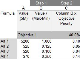
This is where we multiply the ranking for each objective by the priority of the objective. In both Ideal mode and Grid mode, we simply multiply the normalized rankings derived in Step 1 by the priority of its covering objective, e.g. (O1 x A1), (O1x A2), etc. where O1 is the priority of Objective 1 and An is the normalized ranked value for Alternative n. This is done for each alternative and for each objective. Table 1 below shows the calculation for Steps 1 and 2 in Ideal mode for Objective 1 (which has a priority of 40%).
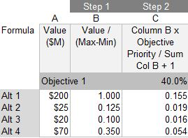
In Distributed mode, the approach is different because of the way the weights are distributed amongst the alternatives. We perform the same normalization calculation as above (Step 1 & 2), but the result is then divided by the sum of the normalized rankings + 1 (the '1' being introduced as the ideal alternative), e.g (O1 x A1) / (ΣAn-o1 + 1), where ΣAn-o1 is the sum of the normalized ranked values for Objective 1.
Step 3: Sum the weighted alternatives
The next step is simply, for each alternative, sum the values from Step 2 for each objective. For the IDeal and Grid mode, this is:
IPA1 = (O1 x A1) + (O2x A1) + ...
where IPA1 is the interim ranking (or priority) of Alternative 1. Note that we call it an interim priority because some additional normalization is required after in order to calculate the final priorities. For the Distributed mode, this is
IPA1 = (O1 x A1) / (ΣAn-o1 + 1) + (O2 x A1) / (ΣAn-o2 + 1) + ...
Step 4: Calculate final alternative priorities
For the Grid mode, the resulting IPAnis the final priority. This in itself is somewhat meaningless (because the priorities don't add up to 100%), so they need to be further normalized.
In the Ideal mode two normalization steps are required. First, the values derived in Step 3 are adjusted by assigning the winner the value '1', and all other priorities are normalized with respect to the winner. It is this step that preserves the ranking of the alternatives. The resulting values are then normalized in the traditional way such that the totals add up to 100%.
In Distributed mode, the values derived in Step 3 are simply normalized in the traditional way such that the totals add up to 100%.
To help understand this more, we have provided two files that can be downloaded and manipulated:
File 1: An Excel of the example use in this note, showing the AHP Calculations (download here)
File 2: A decisionAccelerator model of the above example (download here)
Note: Only people with decisionAccelerator installed should download File 2 as it requires the decisionAccelerator engine.